Duplicates in data? Excel is a better option!!

Here’s my first post for my blog. I’m so excited.

I’ve chosen this topic “Duplicates” as my first topic. It is quite common that we work with data that has duplicates. It is not always common how we treat duplicates each time we come across. Thankfully Excel has inbuilt tools and functions to figure out duplicates. I want to share the ways I use to deal with them.

There are times when you want to:

            1.  Identify duplicates in data

            2.     Keep only unique data

1.            Identifying duplicates in data

       1.1.    Using Countif function

Just as an example, in a list of names I want to know how many names are repeated. Here is how I use countif.

Below table starting from cell A1.

Names

Praveen

Raju

Amar

Murali

Narendar

Saravana

Praveen

               

Here is the countif formula in column B to know the duplicates. In cell B2 type formula =COUNTIF ($A$2:$A$8, A2) and copy it down till you have your data.

Names	Duplicates
Praveen	=COUNTIF($A$2:$A$8,A2)
Raju	=COUNTIF($A$2:$A$8,A3)
Amar	=COUNTIF($A$2:$A$8,A4)
Murali	=COUNTIF($A$2:$A$8,A5)
Narendar	=COUNTIF($A$2:$A$8,A6)
Saravana	=COUNTIF($A$2:$A$8,A7)
Praveen	=COUNTIF($A$2:$A$8,A8)

Now the result looks like:   

         

Names	Duplicates
Praveen	2
Raju	1
Amar	1
Murali	1
Narendar	1
Saravana	1
Praveen	2

Now you know where the duplicates are. In addition, one can also do a conditional formatting to colour the duplicate names. We will discuss conditional formatting in next section.

        1.2.    Using a pivot table

        

         Using the example from above.

          

Names

Praveen

Raju

Amar

Murali

Narendar

Saravana

Praveen

Short cut in excel ALT+D+P takes you to Pivot table wizard.

Navigation in excel 2007: Select your data in the worksheet, click Insert on the toolbar, PivotTable.

Navigation in Excel 2003: Click Data on the toolbar, PivotTable and PivotChartReport.

Choose where you want to put the Pivot table report and click finish.  Add “Names” field to row labels and also to data area / labels to show the count.

Row Labels	Count of Names
Amar	1
Murali	1
Narendar	1
Praveen	2
Raju	1
Saravana	1
Grand Total	7

Now you know where the duplicates are. In addition, one can also do a conditional formatting to colour the duplicate names. We will discuss conditional formatting in next post.

       1.3.    Conditional formatting

In Excel 2003, select all your data. In our example, it is A1:A8.

Click Format on toolbar and Conditional Formatting. Set the dropdown to Formula is and copy/type this formula next =COUNTIF ($A$1:$A$8, $A1)>1. Now choose the format you like and click Ok. You will see the duplicates are formatted.

In Excel 2007, There is a simple option instead of typing a formula (You can still use the formula but there is an easy option) to figure out duplicate values in the range. Here we go, select the range, Click Home on the toolbar. Under Styles, click on Conditional Formatting, Highlight Cells Rules, Duplicate Values.

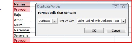
             Select Duplicate in the duplicate/unique dropdown and choose the format you like in      

             the Values with dropdown and click Ok.

             I’m sure subtotals are also a way but that is no easy option compared to any of the 

             above. We need to sort the data first and do the subtotals to know the unique values 

             and count of duplicates next to it. Let me know if any of our readers use sub-totals for 

             this purpose. If yes, then why?

2.       Unique data

From the above techniques, Pivot table is one way that gives unique values. So, am not including that technique again.

       2.1.    Advanced Filter

             Shortcut in Excel ALT+D+F+A

             In Excel 2003, select Data, click on Advanced Filter and choose List range (Your    

             data range), click

  on radio button Copy to another location , check the Unique 

             records only check box and choose 

where you want to copy unique values to.

            

P.S: This option assumes you have headers. Hence first row is not taken as data in the list you choose.

P.P.S:  If you do not choose Copy to another location radio button, then it filters and shows only unique values.

              In Excel 2007, select Data on toolbar, click on Advanced and choose List range 

              (Your data range), click on radio button Copy to another location , check the 

              Unique records only check box and choose where you want to copy unique values 

              to.

             

P.S: This option assumes you have headers. Hence first row is not taken as data in the list you choose.

P.P.S:  If you do not choose Copy to another location radio button, then it filters and shows only unique values.

       2.2.    Remove Duplicates

         This option is in Excel 2007. Not sure with Excel 2010 (Have not used this yet). 

         In Excel 2007, Select your range and select Data on toolbar. Under Data Tools 

         click on Remove Duplicates

               

Select columns you need to remove duplicates and if applicable check on My Data has headers check box and say Ok.

You will be shown a message box like below with duplicates found and removed.

            

P.S. Duplicates are deleted from the list you choose.
Note: For simplicity sake I just took names (One column) of my friends as data. It could be more complicated data (with multiple columns). All the techniques are valid for such data. Write to me if you face any issues. I’ll be glad to help you.

Hope this is all useful. These are the techniques I use (I have not shared my VBA script yet but will share that soon) to remove duplicates/keep unique values. All said, I invite all your opinions and suggestions on this write-up. Also, please share if you use any other techniques or I skipped/missed anything.